17. Divergence, Curl and Potentials
c. The Curl Operator
2. Geometric Interpretation of the Curl
The curl of a vector field measures how much the vector field is rotating at each point. More concretely, if the vector field \(\vec V\) is the velocity field of a fluid, then the curl of the velocity field, \(\vec\nabla\times\vec V\), is also a vector field and we need to give a description of its magnitude and direction at each point. The direction of the curl is the axis of rotation. The magnitude of the curl is the rate at which the fluid is rotating. The direction of rotation is determined by the right hand rule. In particular, if you hold your right hand in a fist and point your thumb along the direction of the curl, then the fluid rotates in the direction of your fingers, i.e. counterclockwise as seen from the tip of your thumb.
When we discussed the Geometric Interpretation of the Divergence, it was easier to visual the vector field in \(\mathbb R^2\). We would like to do the same for the curl. However, just as the cross product of two vectors is only defined in \(\mathbb R^3\), likewise, the curl of a vector field is (officially) only defined in \(\mathbb R^3\). Luckily, we have the following work-around: Given a vector field in \(\mathbb R^2\): \[ \vec F=\left\langle F_1, F_2\right\rangle \] we observe that \(F_1\) and \(F_2\) are only functions of \(x\) and \(y\). Then we can regard this vector field as a vector field in \(\mathbb R^3\) whose third component is \(0\) and whose first and second components are only functions of \(x\) and \(y\). Thus, \[ \vec F=\left\langle F_1(x,y), F_2(x,y), 0\right\rangle \] When we compute the curl, we get \[\begin{aligned} \text{curl} \vec F &=\vec\nabla\times\vec F =\begin{vmatrix} \hat\imath & \hat\jmath & \hat k \; \\ \partial_x & \partial_y & \partial_z \; \\ F_1(x,y) & F_2(x,y) & 0 \; \end{vmatrix} \\ &=\hat\imath(0-0) -\hat\jmath(0-0) +\hat k (\partial_x F_2-\partial_y F_1) \\ &=\left\langle 0, 0, \partial_x F_2-\partial_y F_1\right\rangle \end{aligned}\] which only has a \(z\)-component: \[ (\vec\nabla\times\vec F)_z=\partial_x F_2-\partial_y F_1 \] This means that the curl points along the positive \(z\)-axis if \(\partial_x F_2-\partial_y F_1 \gt 0\) and the negative \(z\)-axis if \(\partial_x F_2-\partial_y F_1 \lt 0\). We would like to see that:
If \(\ \partial_x F_2-\partial_y F_1 \gt 0\ \) then the fluid flows counterclockwise.
and:
If \(\ \partial_x F_2-\partial_y F_1 \lt 0\ \) then the fluid flows clockwise.
This would justify the right hand rule.
To understand which direction the vector field is rotating, we first look at
a vector field in the \(xy\)-plane with only one component.
In the figures below, use your mouse to drag the center of the circle to
move it, or drag the circumference to change the radius.
Consider the vector field:
\[
\vec F=\left\langle 0, F_2(x,y), 0\right\rangle
\]
In the figure on the left \(\partial_x F_2 \gt 0\) which means \(F_2\) gets
bigger from left to right. In other words, on each circle, the counterclockwise
blue arrows are bigger.
In this case, \((\vec\nabla\times\vec F)_z=\partial_x F_2-\partial_y F_1 \gt 0\).
In the figure on the right \(\partial_x F_2 \lt 0\) which means \(F_2\) gets
smaller from left to right. In other words, on each circle, the clockwise
red arrows are bigger.
In this case, \((\vec\nabla\times\vec F)_z=\partial_x F_2-\partial_y F_1 \lt 0\).
Now consider the vector field:
\[
\vec F=\left\langle F_1(x,y), 0, 0\right\rangle
\]
In the figure on the left \(\partial_y F_1 \gt 0\) and so
\((\vec\nabla\times\vec F)_z \lt 0\). On each circle,
the red clockwise arrows are bigger.
In the figure on the right \(\partial_y F_1 \lt 0\) and so
\((\vec\nabla\times\vec F)_z \gt 0\). On each circle,
the blue counterclockwise arrows are bigger.
For a vector field with both components, \(\vec F=\left\langle F_1(x,y), F_2(x,y), 0\right\rangle\), the direction of rotation depends on which of \(\partial_x F_2\) or \(\partial_y F_1\) is bigger.
The plot shows a vector field of the form: \[ \vec F=\left\langle F_1(x,y), F_2(x,y), 0\right\rangle \] Determine the regions in the plot where \((\vec\nabla\times\vec F)_z \gt 0\) and where \((\vec\nabla\times\vec F)_z \lt 0\).
Imagine drawing a small circle at each point. Are the arrows pointing counterclockwise bigger or smaller than those pointing clockwise?
\((\vec\nabla\times\vec F)_z \gt 0\) in the blue region, quadrants
I and II.
\((\vec\nabla\times\vec F)_z \lt 0\) in the red region, quadrants
III and IV.
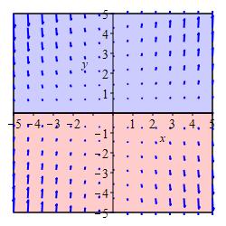
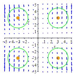
We draw circles at a bunch of points. Those centered in quadrants I and II have bigger arrows pointing counterclockwise than clockwise. So \((\vec\nabla\times\vec F)_z \gt 0\) there. Those centered in quadrants III and IV have bigger arrows pointing clockwise than counterclockwise. So \((\vec\nabla\times\vec F)_z \lt 0\) there. See the Answer for a summary plot.
The plot shows a vector field of the form: \[ \vec F=\left\langle F_1(x,y), F_2(x,y), 0\right\rangle \] Determine the regions in the plot where \((\vec\nabla\times\vec F)_z \gt 0\) and where \((\vec\nabla\times\vec F)_z \lt 0\).
Imagine drawing a small circle at each point. Are the arrows pointing counterclockwise bigger or smaller than those pointing clockwise?
\((\vec\nabla\times\vec F)_z \gt 0\) in the blue region, above
the diagonal.
\((\vec\nabla\times\vec F)_z \lt 0\) in the red region, below
the diagonal.
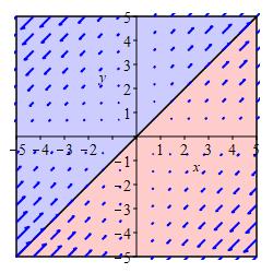
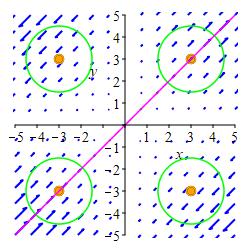
We draw circles at a bunch of points. Those centered along the line \(y=x\) have as many big arrows going clockwise as counterclockwise. So \(\vec\nabla\cdot\vec F=0\) there. Those centered above and to the left of this line have bigger arrows pointing counterclockwise. So \(\vec\nabla\cdot\vec F \gt 0\) there. Those centered below and to the right of this line have bigger arrows pointing clockwise. So \(\vec\nabla\cdot\vec F \lt 0\) there. See the Answer for a summary plot.
A fuller geometrical discussion of the curl uses an integral to sum up the arrows going around the boundary circle and takes the limit as the radius goes to \(0\). This discussion appears in the chapter on the Interpretation of Divergence and Curl.
Heading
Placeholder text: Lorem ipsum Lorem ipsum Lorem ipsum Lorem ipsum Lorem ipsum Lorem ipsum Lorem ipsum Lorem ipsum Lorem ipsum Lorem ipsum Lorem ipsum Lorem ipsum Lorem ipsum Lorem ipsum Lorem ipsum Lorem ipsum Lorem ipsum Lorem ipsum Lorem ipsum Lorem ipsum Lorem ipsum Lorem ipsum Lorem ipsum Lorem ipsum Lorem ipsum